




How to Highlight in Excel: Cells, Text Inside a Cell, Duplicates and Conditional Formatting Rules
Excel has no highlighter button for text, so highlighting there means one of three things: fill color, font color, or a rule that colors cells for you.
in short
To highlight in Excel, select the cells, go to the Home tab and pick a color from the arrow next to Fill Color. To color only some text in a cell, select those characters and use Font Color. To highlight automatically, use Home > Conditional Formatting > Highlight Cells Rules, for example Duplicate Values.
If you are looking up how to highlight in Excel, the first thing to know is that Excel does not work like Word. Microsoft says plainly that Excel does not provide a button to highlight all or part of the data in a cell. Instead you color the whole cell with Fill Color, color some of the characters with Font Color, or let a conditional formatting rule color cells that meet a condition, such as duplicates or values over a limit. Below are Microsoft's steps for each method on Windows, Mac and the web, how to remove each, and a worked example.
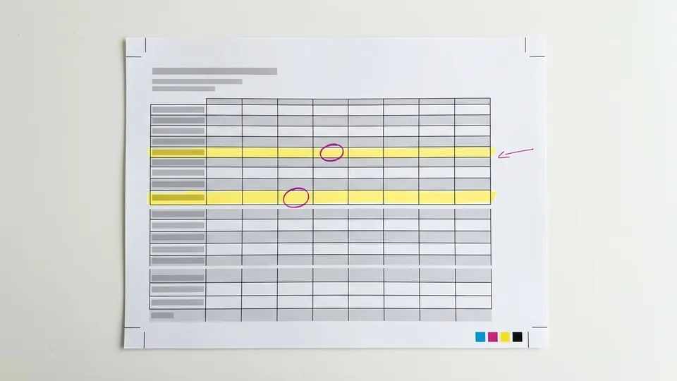
How to highlight in Excel: three methods
Choose by what the color should do. A fill or font color stays until you remove it; a conditional formatting rule recalculates, so the color moves when the data changes.
| Method | Where it is | What it colors | Changes with the data? | How to remove it |
|---|---|---|---|---|
| Fill Color | Home > arrow next to Fill Color | The whole cell background | No | Fill Color > No Fill, or Clear > Clear Formats |
| Font Color | Home > Font group > Font Color | Selected characters, even part of a cell | No | Set the font color back |
| Custom cell style | Home > Cell Styles > New Cell Style | Cells you apply the style to | No | Apply a different style |
| Conditional formatting | Home > Conditional Formatting | Cells that meet a rule | Yes | Conditional Formatting > Clear Rules |
Highlight cells with Fill Color
In Excel, a highlight is a cell color, not a mark on the words.
Microsoft's page on how to add or change the background color of cells in Excel says you can highlight data in cells by using Fill Color. The steps for Excel for Windows:
Select the cells
Drag across the cells, or click the Select All button to color the whole worksheet. Microsoft notes that a whole-sheet color hides the gridlines.
Open Fill Color
On the Home tab, select the arrow next to Fill Color, or press Alt+H, H.
Pick a color
Choose a color under Theme Colors or Standard Colors. For anything else, select More Colors.
Repeat the last color quickly
Select the Fill Color button itself, not the arrow, to apply the color you used most recently.
For patterns, use the Fill tab of the Format Cells dialog (Ctrl+Shift+F). Microsoft warns that pattern fill effects are not available in Excel for the web and will not appear in the browser.
Excel for Mac
Microsoft's guide to highlighting cells in Excel for Mac gives the same idea with the Mac ribbon: select the cells, then on the Home tab, in the Font group, click Fill Color. To use a different color, click the arrow next to Fill Color first.
Excel for the web
In the browser, select the cells, then on the Home tab select Fill Color and pick a color. Solid fills work; pattern fills, as noted above, do not display.
Highlight text inside a cell
Because there is no text highlighter, the closest match for a word or two inside a cell is a different font color or format. The Mac guide describes it: to select part of the data, double-click the cell, select the characters you want, then on the Home tab, in the Font group, click the arrow next to Font Color and choose a color. Bold, Italic and Underline work on a partial selection in the same way.
Save a highlight as a cell style
If you highlight with the same color all the time, save it. Microsoft's Mac guide gives the steps, which match the Windows ribbon: on the Home tab, in the Styles group, click Cell Styles, then New Cell Style. Name the style, click Format, choose a color on the Fill tab, and click OK twice; the style appears under Custom. To copy a highlight to many cells, select a highlighted cell, double-click Format Painter on the Home tab, then select each cell you want to mark; click Format Painter again to stop.
Highlight cells automatically with conditional formatting
Microsoft's page on how to use conditional formatting to highlight information describes the feature as rules that set the format of cells based on their values. Its example is coloring products with fewer than 10 items on hand in yellow.
Select the range
Select the cells the rule should check: a range, a named range or an Excel table.
Open Highlight Cells Rules
On the Home tab, in the Styles group, click the arrow next to Conditional Formatting, then Highlight Cells Rules.
Pick a comparison
Choose a command such as Greater Than, Between, Equal To, Text that Contains or A Date Occurring.
Enter the value and a format
Type the value to compare against, choose a format, and confirm. Excel colors every cell that meets the condition.
For anything the built-in rules do not cover, choose Conditional Formatting > New Rule, then the rule type Use a formula to determine which cells to format. Microsoft's conditions: the formula has to start with an equal sign (=) and return TRUE or FALSE. Click Format to choose the fill, font or border that appears when the formula is true. Microsoft also notes that a cell whose formula returns an error is not formatted by the rule.
To edit, reorder or delete rules later, Home > Conditional Formatting > Manage Rules opens the Conditional Formatting Rules Manager.
In Excel for the web, the rules live in a Conditional Formatting pane: choose Home > Styles > Conditional Formatting > New Rule, check the Apply to range, choose a Rule Type (Formula is one), and select Done.
Highlight duplicates in Excel
Duplicates are the most common reason to highlight a column. Microsoft's page on how to find and remove duplicates recommends highlighting them first, so you can review them before deleting anything.
- Select the cells you want to check.
- Select Home > Conditional Formatting > Highlight Cells Rules > Duplicate Values.
- In the box next to values with, pick the formatting for the duplicates, then select OK.
Microsoft notes one exception: Excel cannot highlight duplicates in the Values area of a PivotTable report. If you then want the copies gone, Data > Remove Duplicates deletes them. Microsoft warns that this deletion is permanent and suggests copying the original data to another worksheet first, removing any outlines or subtotals, and treating the reported counts with care, because they can include empty cells and spaces.
How to remove highlighting in Excel
- Fill color, straight away. Select Undo.
- Fill color, later. Select the cells, then Home > the arrow next to Fill Color > No Fill. Microsoft's web steps also give Clear > Clear Formats, which removes all formatting from the selection, not only the color.
- Conditional formatting on a range. Select the cells, then Home > Conditional Formatting > Clear Rules > Clear Rules from Selected Cells.
- Conditional formatting on the whole sheet. Home > Conditional Formatting > Clear Rules > Clear Rules from Entire Sheet. In the web version, Manage Rules also has a Delete All Rules button.
A worked example: a reading log
The sheet below is a sample made up for this example: a class reading log with names in column A and pages read in column B, rows 2 to 6.
| Row | A: Student | B: Pages read | Highlight it gets |
|---|---|---|---|
| 2 | Ana | 142 | Green (Greater Than 100); name marked by Duplicate Values |
| 3 | Ben | 18 | Whole row light red: formula rule |
| 4 | Ana | 142 | Green (Greater Than 100); name marked by Duplicate Values |
| 5 | Chloe | 64 | None |
| 6 | Dev | 11 | Whole row light red: formula rule |
- Duplicates. Select A2:A6 and apply Duplicate Values. Both Ana cells turn color, so you can check whether the second entry is a mistake before removing it.
- A threshold. Select B2:B6 and apply Highlight Cells Rules > Greater Than with 100. Rows 2 and 4 turn green.
- A whole row. Select A2:B6, choose New Rule > Use a formula to determine which cells to format, and enter =$B2<20. The dollar sign fixes the column, so each row checks its own page count, and rows 3 and 6 turn light red.
Change Ben's 18 to 40 and his row loses its color at once. That is the difference between a rule and a fill.
Pitfalls when highlighting in Excel
- Looking for a highlighter button. There is none for cell text. Use Fill Color for cells and Font Color for characters.
- Colors that do not print. Microsoft says cells will not print in color if the sheet is set to Black and white or Draft quality. Clear both in Page Layout > Page Setup, on the Sheet tab.
- Patterns that vanish online. Pattern fills do not show in Excel for the web. Use solid fills in shared workbooks.
- Deleting before checking. Remove Duplicates is permanent. Highlight first, review, and keep a copy.
Tips for clearer spreadsheet highlights
- Fix a key. Decide what each color means before you start and write the key in a cell above the table. The same idea is set out in the highlighter color-code system.
- Know where Excel differs. In Word, highlighting is a text feature; the guide to highlighting in Word covers it, and highlighting in Google Docs works the same way.
Highlighting in Excel comes down to choosing the right kind of color: Fill Color for cells you mark by hand, Font Color for a word inside a cell, and conditional formatting for anything the data should decide, duplicates included. Remove each with its own control, No Fill or Clear Rules, and keep a key so the colors mean the same thing to every reader. The other highlighting and annotation guides cover documents, PDFs, slides and the web.
Common questions
Is there a highlight button in Excel?
No. Microsoft states that, unlike Word, Excel does not provide a button to highlight all or part of the data in a cell. You can mimic a highlight by filling the cell with color, save that color as a custom cell style, or change the font color of the characters you want to stand out.
How do I highlight part of the text in a cell?
Double-click the cell, select just the characters you want, then on the Home tab use the arrow next to Font Color to pick a color. Bold, Italic and Underline also work on a partial selection. Fill Color always colors the whole cell, so it cannot mark a single word.
How do I highlight duplicates in Excel?
Select the cells, then choose Home > Conditional Formatting > Highlight Cells Rules > Duplicate Values. Pick a format in the box next to values with and select OK. Every repeated value is colored. Microsoft notes this does not work in the Values area of a PivotTable report.
How do I highlight a whole row based on one cell?
Select the rows, choose Home > Conditional Formatting > New Rule, then Use a formula to determine which cells to format. Enter a formula that starts with an equal sign and returns TRUE or FALSE, such as =$B2>100, and set a fill under Format. The dollar sign keeps every row checking column B.
Why won't my highlight go away in Excel?
The color is probably set by a conditional formatting rule, not by Fill Color, so No Fill has no effect. Select the cells and choose Home > Conditional Formatting > Clear Rules > Clear Rules from Selected Cells, or open Manage Rules to find and delete the rule that applies.
Sources
sign-off
Checked against its sources and signed before it went out.
Nora Feld
Editor · reviewed 2 Nov 2026